Starting from the original reference, Mixture of Experts Explained, this note keeps three questions in view: what is an expert, how does a router assign inputs, and what does sparse computation save—or leave unsaved?
Chapter 1: Not every input needs the whole network↗
A classic early contribution to mixture of experts (MoE) is Jacobs and colleagues’ Adaptive Mixtures of Local Experts (1991). Separate networks learn to handle different input cases, with a gating network helping determine their combination. The idea does not depend on Transformers: the 2017 sparsely gated MoE work applied it to LSTM language models.
In many Transformer MoEs, some dense feed-forward networks (FFNs) are replaced by a bank of experts and a router. The experts are usually FFNs themselves. “Expert” names a computational module; it does not guarantee that each module specializes in a neatly named human topic.
The central idea is to activate only part of the expert bank for an input, rather than average the answers of several complete models. The model can have many parameters while using few experts for each token.
Chapter 2: How do experts and routers work together?↗
2.1 From gates to a sparse combination↗
For a token representation at a particular layer, let be expert ’s output, the set selected by the router, and its gate weight. A common combination takes the form:
The number of experts, how many are selected for a token, and whether selected weights are renormalized are architectural choices. A token may go to one expert or several, and different tokens may take different routes.
2.2 Switch: select one, retain its gate value↗
Switch Transformer uses top-1 routing. Setting aside capacity overflow and other implementation details, the core of its sparse FFN layer is:
Here, is the router’s weight matrix, and its probability for expert . The selected gate value comes from a softmax over all experts; selecting only one does not automatically make its weight 1. This equation describes the sparse FFN sublayer, not the output of an entire Transformer block.
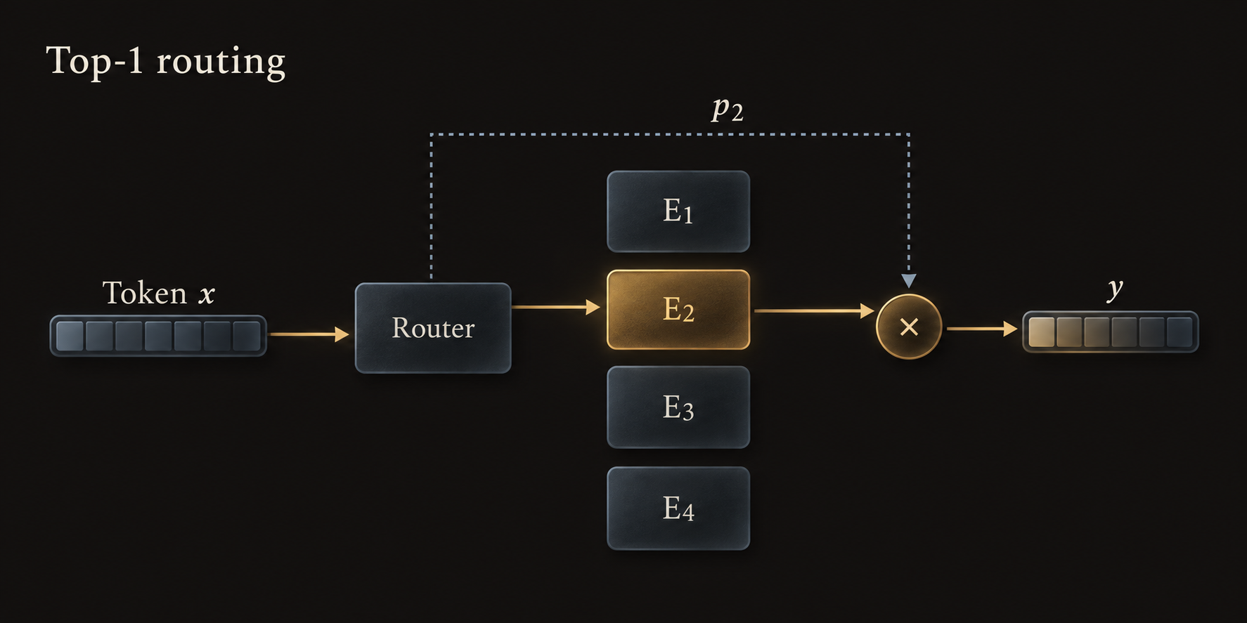
The original figure used “More” and “Parameters” to illustrate different routes. This diagram simplifies the example to one token: select , compute its output, then multiply by gate value . Every token has its own routing decision; is not permanently assigned to one particular word.
The router and experts learn under the overall training objective, but routing creates an allocation problem. If too many tokens go to a few experts, others may receive too little training. Switch uses an auxiliary load-balancing loss and limits expert capacity. In that implementation, overflow tokens can skip the expert computation in this layer and continue through the residual path. They do not disappear from the sequence.
Chapter 3: More capacity does not make speed free↗
The original note summarized the trade-off as faster training and inference, but greater memory demands and harder fine-tuning. A more precise reading needs to specify the comparison:
| Quantity | Opportunity offered by sparse MoE | Conditions that still matter |
|---|---|---|
| Computation per token | Avoid executing every expert | Routing, other sublayers, and communication still cost resources |
| Training efficiency | May outperform a dense baseline at a given resource and quality target | Specify hardware, data, target quality, and training recipe |
| Inference speed | Activating fewer parameters can help at the same total parameter count | Actual latency also depends on batching, load balancing, and inter-device transfers |
| Memory and fine-tuning | More capacity to learn from; successful instruction-tuned examples exist | Inactive weights still require storage; resource layout and adaptation methods matter |
For a concrete distinction, the 2024 Mixtral 8x7B has eight experts per MoE layer and selects two for each token. The paper reports about 47B total parameters and 13B active parameters per token during inference. That describes one configuration: “8×7B” is not simply eight independent full models added together, and not every MoE uses top-2 routing.
Experts can be distributed across devices, so all weights need not reside on one GPU. But not computing with a weight on this occasion does not remove the need to store it. Deployment must account for parameter storage, active computation, and data movement together.
Total parameters, active parameters, and runtime are three different quantities. Separating them makes the actual trade-off behind a larger model easier to see.