Advanced visualisation · I: the many forms of text

Chapter 1: Why turn text into a picture?↗

Text visualization can begin with four questions. How can a reader grasp the outline of a document? Compare documents or follow their evolution? Find an entry point for grouping and topic exploration? Relate textual patterns to other data?

A picture does not guarantee faster or more accurate reading. It brings some relations forward while hiding others. Decide what needs to become visible before choosing how to compress the text.

1.1 What kind of data is text?↗

Web pages, articles, logs, books, email, comments, source code and tags can all be documents. Organizing them by author, time, community or task produces different collections.

Characteristic	Implication for visualization
Abstraction	Characters need not resemble what they refer to
Sequence	Word order can change meaning; prose is usually read sequentially
Multiple levels	Words, sentences, paragraphs, grammar and typography offer different units of analysis
Variation across groups and settings	The same word can serve different purposes across communities, genres and contexts

1.2 More than too many words↗

Challenge	What must be decided?
High dimensionality	Which terms, relations and levels should survive?
Keywords	Are frequency, distinctiveness and descriptiveness the same thing?
Context	How much text preserves negation, modification and whom a statement addresses?
Meaning	How should ambiguous forms, synonyms and metaphor be handled?
Access to the source	Can readers return from the view to the relevant passage?
Domain structure	Does a classification or ontology require additional domain knowledge?

Terms can be counted as categories without reducing their meanings to equality tests. Paris, New York and Madrid share a city category; that list alone establishes no statistical correlation. January, February and March have a calendar order, but arbitrary vocabularies have no natural ordering. Inflection is also different from synonymy, antonymy and hierarchical relations.

Chapter 2: Processing is not one fixed pipeline↗

Tokenization, entity recognition, stemming and lemmatization are different operations. They can be combined without always running every step in one order. Stemming and lemmatization are often alternatives chosen for a task.

Operation	Purpose	Example and boundary
Tokenization	Segment characters into tokens while retaining alignment with the source	“a sentence” can yield two tokens; punctuation may also be retained
Filtering	Decide whether to remove stop words, numbers or symbols	This is not the definition of tokenization; negation and prepositions may be the object of study
Named entity recognition	Identify spans referring to people, organizations, places and other categories	James Bond may be tagged as a person; categories depend on the model and annotation scheme
Stemming	Merge some forms through rules; the result need not be a complete word	fishing and fished may reduce to fish; rules differ
Lemmatization	Recover a base form using dictionaries, rules or models	went can map to go; results may depend on part of speech and context
Vocabulary indexing	Assign computational identifiers to terms	The IDs for go and good encode no magnitude, distance or semantic order

spaCy’s linguistic-feature documentation distinguishes these operations. Informal text, abbreviations, names and multiword entities need separate attention. Preserve surface forms or source offsets for presentation: a stem generally cannot be uniquely reversed.

Tools such as Gensim and spaCy can help implement the processing, but the unit of analysis comes first. If the question concerns “X and Y,” deleting and at the start removes the very connection the later network is meant to find.

Chapter 3: Bags, matrices and clouds↗

3.1 A document as a vector↗

A basic bag-of-words representation counts terms while discarding their positions. It may use unigrams or extend to n-grams. The latter preserve local order without preserving the arrangement of all phrases in the document. Omitting order from a representation does not assert that terms are statistically independent.

For $D$ documents and a vocabulary of $V$ terms, a document–term count matrix can be written as:

Rows represent documents and columns represent terms. scikit-learn’s text-feature guide uses this convention. The original note’s transposed layout below makes the plays easier to compare. Its values come from a teaching table in the related lecture, rather than a corpus recounted for this revision.

Term	Antony and Cleopatra	Julius Caesar	The Tempest	Hamlet	Othello	Macbeth
Antony	157	73	0	0	0	0
Brutus	4	157	0	1	0	0
Caesar	232	227	0	2	1	1
Calpurnia	0	10	0	0	0	0
Cleopatra	57	0	0	0	0	0
mercy	2	0	3	5	5	1
worser	2	0	1	1	1	0

Counts are only one weighting scheme. Relative frequency, $X_{dv}/\sum_uX_{du}$, can help compare documents of different lengths when the denominator is positive. TF–IDF answers another question. Frequency, distinctiveness and usefulness to a reader are not interchangeable.

3.2 Word clouds: visibility has a cost↗

Tag clouds commonly encode frequency or another weight through type size. They can suggest a useful query without supporting precise comparisons.

What they can support	What they can obscure
Finding prominent terms	Grammar, relations and negation
Forming a query	Size and arbitrary placement are often harder to compare than positions on a shared scale
Quick scanning	Longer words occupy more area without necessarily having greater weight
An overview	Unstable layouts complicate comparisons between documents

3.3 Recovering a modifier↗

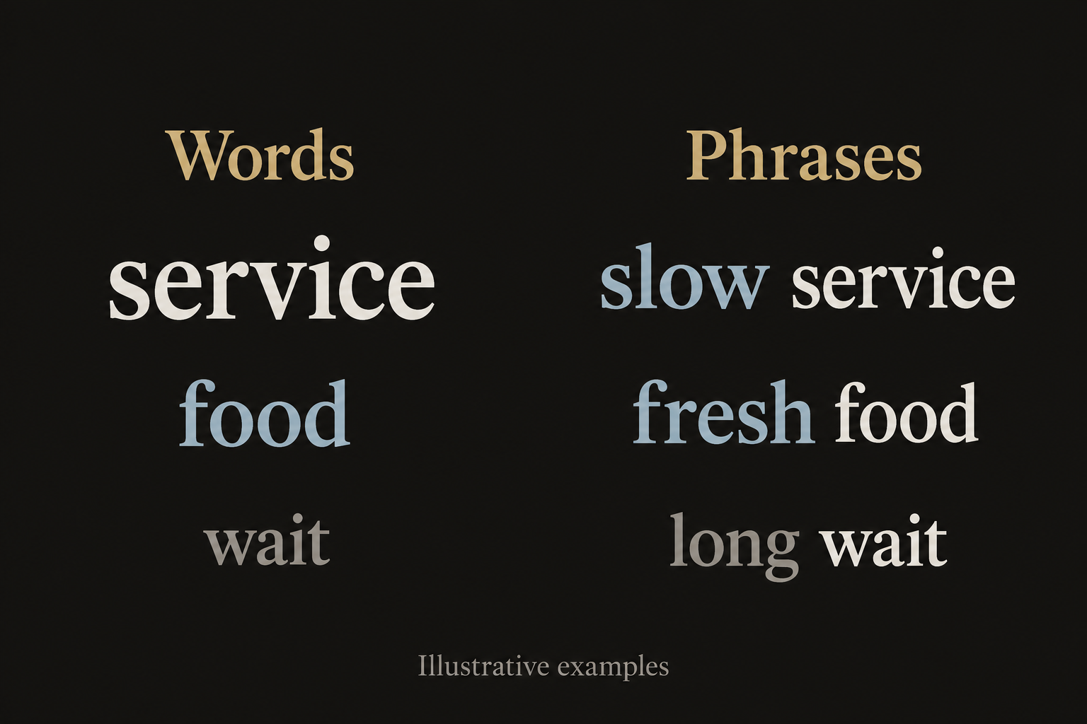
Frequent mentions of “service” do not yet distinguish praise from complaint. “Slow service” retains a relation. Adjective–noun pairs can therefore be useful for summarizing reviews, without being universally superior to bags of words. Extraction can fail, and irony, negation and longer contexts may still be lost.

Chapter 4: Putting local context back↗

4.1 Beyond a matching string↗

Retrieval can show the text around a hit as well as match a query, highlighting the query term within it. Keyword-in-context (KWIC) reconnects occurrence with use. SeeSoft and TileBars offer different historical examples in the related course material; they need not be treated as a current list of ready-to-use software.

The interface should provide a route back to the sentence. Otherwise, a striking word may come from a passage whose negation or quotation marks have disappeared.

4.2 WordTree: where repetition branches↗

Wattenberg and Viégas’s WordTree starts from a query word or phrase and organizes repeated following or preceding sequences as a tree. Shared prefixes merge before branching at different words. This is not a syntactic parse tree or simply a list of fixed-length n-grams.

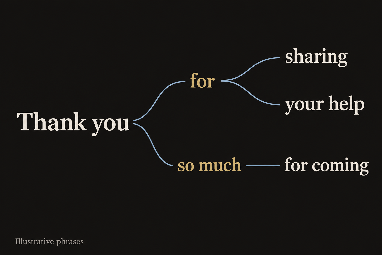
The starting point determines which local structures become visible. Exact matching separates lexical and syntactic variants. Filtering rare branches improves legibility, but the remaining display is no longer the complete distribution. Jason Davies’s interactive implementation offers a way to explore this form of querying.

4.3 Phrase Nets: define the relation first↗

Phrase Nets find a specified relation, such as “X and Y” or “X at Y,” or use the output of syntactic analysis. Matches become a node–link view. In the original design, occurrences can affect node size and pattern position can determine edge direction. Changing the pattern changes the network. See Mapping Text with Phrase Nets.

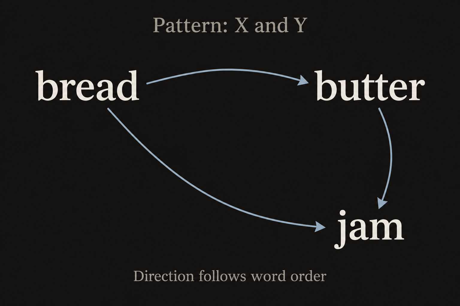
An edge first establishes a match to the chosen relation; it does not automatically establish a causal, psychological or social connection. The extraction rule belongs alongside the graph’s interpretation.

Chapter 5: Documents have positions, versions and participants↗

5.1 Content and interaction↗

Perspective	Relations that may be retained
Within a document	Term position, sequence, paragraphs and hierarchy
Between documents	Similarities or groups computed from explicit features
Layout	Map selected relations into space without assuming every distance has semantic meaning
Interaction	Browse, brush, link views, return to passages and revise query patterns

5.2 Beyond the final version↗

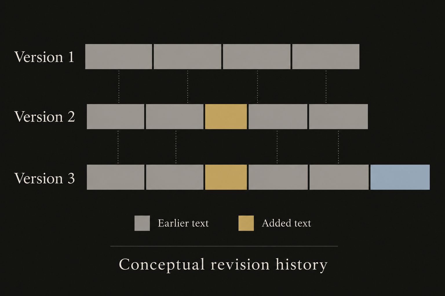
Revision records can reveal when passages were added, removed or retained. Wikipedia’s History Flow and Git histories concern different objects. Animation is one way to present time, rather than a requirement.

The original note illustrated this section with Ben Fry’s The Preservation of Favoured Traces, which follows six editions of On the Origin of Species, rather than Wikipedia edits. The schematic here does not use the book’s data; the original project remains available through the link.

5.3 Conversation: who, what and when↗

Conversations can be examined by sender and recipient, content, time and combinations of these dimensions. Message volume alone does not establish the quality of a relationship. Terms alone may not reveal who is replying to whom.

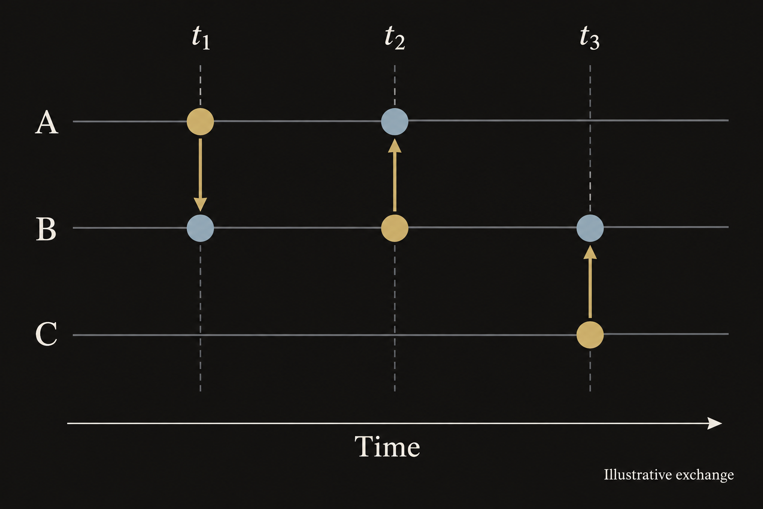
Historical designs include Newsgroup Crowds, AuthorLines, Mountain and Themail. Themail connects the terms in an email correspondence with time and provides access to the original messages. Such designs help formulate more specific reading questions without explaining an entire relationship on its participants’ behalf.

Chapter 6: From collections to latent topics↗

6.1 Comparing side by side↗

Method	Question
Parallel tag clouds	Which terms stand out in each subset, and how does one term recur across groups?
Document projections	Which documents appear close in a low-dimensional view of a specified representation and distance?
Topic-model views	How do documents relate to topics, and topics to terms?

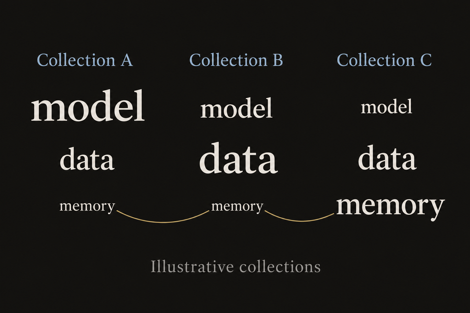
Collins and colleagues’ Parallel Tag Clouds combine a parallel layout with tag clouds and access to individual texts. Comparison involves more than placing independent clouds side by side. Term selection, weight scales, absences and cross-column tracing all affect what can be read.

6.2 LSA: a low-rank approximation↗

Latent semantic analysis (LSA) applies truncated singular value decomposition to a count or TF–IDF matrix. With documents as rows and terms as columns:

The dimensions of $U_k$, $\Sigma_k$ and $V_k$ are $D\times k$, $k\times k$ and $V\times k$. Retaining $k$ singular directions gives a lower-dimensional representation. This use of SVD does not make every direction a directly nameable probabilistic topic.

6.3 LDA: a mixture is not a classification↗

Latent Dirichlet allocation (LDA) is a generative model. A document has a mixture of topics; each topic is a probability distribution over the vocabulary. Given document $d$’s mixture weights $\theta_d$ and topic–term probabilities $\phi$, the probability of a token taking value $v$ is:

Here $\theta_{dk}\geq0$, $\sum_k\theta_{dk}=1$, and each topic satisfies $\phi_{kv}\geq0$, $\sum_v\phi_{kv}=1$. This is a token-level mixture conditional on fixed parameters. Full LDA also includes a prior over document mixtures and inference. A document can involve several topics without being assigned to one exclusive class.

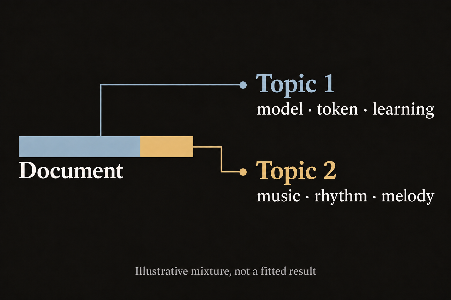
Calling a topic “cats” or “music” is an interpretation of its prominent terms, rather than proof that the model has acquired that concept. LDAvis links a topic overview to term views. Its two-dimensional distances depend on distributional comparisons and projection; the spaces between circles should not be mistaken for meaning itself.

Text has many forms. Each choice determines both what becomes visible and what still requires a return to the words.

第一章：为什么把文字变成图？↗

文本可视化的目的，可以从四个问题展开：怎样更快抓住一份材料的轮廓？怎样比较不同文档，或追踪它随时间的变化？怎样为分组与主题探索提供入口？又怎样把文本模式与其他数据联系起来？

它不一定让阅读更快、更准。图像把某些关系推到眼前，也会把另一些关系藏起来。先问希望看见什么，再决定把文字压缩成什么。

1.1 文本是什么样的数据？↗

网页、文章、日志、书籍、邮件、评论、源代码与标签，都可以成为文档。把它们按作者、时间、社群或任务组织起来，又得到不同的文档集合。

特征	对可视化的影响
抽象	字符本身与所指对象之间并非图像式对应
顺序	改变词序可能改变意思；正文通常需要按顺序阅读
多层结构	词、句子、段落、语法与排版提供不同的分析单位
群体与场景差异	同一词在不同社群、文体和情境里可能承担不同作用

1.2 困难不只在词太多↗

挑战	需要决定什么？
高维度	保留哪些词项、关系与层次？
关键词	高频、区分性与描述性是否是同一件事？
上下文	截取多长，才能保留否定、修饰和说话对象？
语义	同形词、同义词与隐喻怎样处理？
原文入口	读者能否从图返回对应文本，检查解读？
领域结构	分类与本体是否需要额外的领域知识？

词项可以作为类别来计数，却不能因此把语义也当作只有“相同／不同”。Paris、New York、Madrid共享某种城市类别，不等于仅凭这份词表就建立了统计相关；January、February、March有日历次序，也不意味着任意词表都有自然顺序。词形变化是一回事，同义、反义与上下位关系又是另一回事。

第二章：文本处理，不是一条固定流水线↗

分词、实体识别、词干提取与词形还原，是不同的操作。它们可以组合，但并不要求每次按同一顺序全部执行；词干提取与词形还原往往是按任务选择的方案。

操作	做什么	例子与边界
分词	把字符序列切成词元，并保留与原文的对应	“a sentence”可切为两个词元；标点也可以保留
过滤	按任务决定是否删除停用词、数字或符号	它不是分词的定义；否定词与介词可能是研究对象
命名实体识别	标出人名、机构、地名等文本跨度	James Bond可标为人名；具体类别依模型与标注方案而定
词干提取	用规则合并一些词形，输出未必是完整单词	例如将fishing、fished归为fish；不同规则可能不同
词形还原	结合词典、规则或模型，恢复词元的基本形式	went可还原为go；结果可能依赖词性与上下文
词表索引	为词项分配可计算的编号	go与good的编号不表示大小、距离或语义先后

spaCy的语言处理文档区分了这些操作。非正式文本、缩写、专名和跨词实体，需要单独检查。展示结果时，应保留原词或原文位置；词干通常不能被唯一地“反向还原”。

Gensim、spaCy等工具可以帮助实现处理，选择它们之前仍需明确分析单位。若目标是看“X and Y”的用法，一开始就删除and，后面的网络便失去了要寻找的连接。

第三章：词袋、矩阵与词云↗

3.1 把文档写成向量↗

最简单的词袋表示，按词项统计出现次数，舍弃它们在文档中的位置。它可以只用unigram，也可以扩展为n-gram；后者保留局部词序，却仍不保留所有短语在全文中的安排。表示中没有词序，不等于词与词在统计上独立。

设有$D$份文档、$V$个词项，一个文档—词项计数矩阵可以写为：

每一行对应文档，每一列对应词项。scikit-learn的文本特征说明采用这种行列约定；下面为便于对照戏剧，采用转置展示。数值来自相关课程讲义中的教学例表，不是本次重新统计的语料结果。

词项	Antony and Cleopatra	Julius Caesar	The Tempest	Hamlet	Othello	Macbeth
Antony	157	73	0	0	0	0
Brutus	4	157	0	1	0	0
Caesar	232	227	0	2	1	1
Calpurnia	0	10	0	0	0	0
Cleopatra	57	0	0	0	0	0
mercy	2	0	3	5	5	1
worser	2	0	1	1	1	0

词频只是权重的一种。比较长短不一的文档时，可以考虑相对频率$X_{dv}/\sum_uX_{du}$，分母须大于零；TF–IDF等加权又回答不同的问题。出现得多、能区分文档、对读者有意义，不能直接画等号。

3.2 词云：醒目，也有所遮蔽↗

标签云常用字号编码频率或其他权重。它适合提供检索线索，但未必适合精确比较。

可以帮助什么	容易漏掉什么
初步找到突出的词	词之间的语法、关系与否定
形成下一步查询	大小与位置往往不如共同刻度上的位置容易比较
快速扫描	长词占据更大面积，未必代表更大权重
形成概览	不稳定的布局让跨文档比较变难

3.3 从单词到修饰关系↗

“service”出现很多次，尚不能说明人们在称赞还是抱怨。“slow service”保留了一个关系；形容词—名词对因此可以成为评论摘要的一种选择。它并非普遍优于词袋：提取会出错，反讽、否定与更长的上下文也仍可能丢失。

第四章：把局部语境接回来↗

4.1 查询之外，保留前后文↗

信息检索不仅要匹配字符串，也可以显示命中位置附近的文本，把查询词突出出来。keyword-in-context（KWIC）的价值，正是把“出现过”接回“怎样出现”。SeeSoft、TileBars等历史设计可作为相关课程资料中的不同例子，不必被当作今天仍可直接使用的软件清单。

界面应保留返回原句的入口。否则一个醒目的词，可能只是一段被截掉否定或引述标记的话。

4.2 WordTree：重复如何分叉？↗

Wattenberg与Viégas的WordTree从搜索词或短语出发，把后续或前置的重复序列组织成树。共同前缀先合并，在不同词处再分叉；它不是语法分析树，也不只是一张固定长度n-gram列表。

起点决定能看见哪些局部结构。精确词项匹配也会把近义或句式变体分开；若过滤罕见分支，画面更清楚，却不能把剩余分支直接当作完整分布。可在Jason Davies的交互实现中体会这种查询方式。

4.3 Phrase Nets：先定义什么算“有关”↗

Phrase Nets寻找指定关系，如“X and Y”“X at Y”，也可以使用句法分析结果，再用节点—链接图呈现匹配。原设计中，次数可影响节点大小，模式中的位置可决定边的方向；不同模式会得到不同的网络。相关方法见Mapping Text with Phrase Nets。

一条边首先证明符合了所选关系，不会自动证明两个概念在因果、心理或社会意义上相连。 网络的读法需要与提取规则一起交代。

第五章：文档也有位置、版本与参与者↗

5.1 内容与交互↗

分析角度	可以保留的关系
文档内部	词项位置、顺序、段落与层级
文档之间	按明确特征计算的相似性或分组
布局	将选定的关系映射为空间，而不是默认所有距离都有语义
交互	浏览、刷选、联动、返回原文，以及修改查询模式

5.2 演变：不只看最终版本↗

版本记录可以显示何时加入、删去或保留了哪些片段。维基百科的History Flow与Git历史提供不同的分析对象；动画也只是呈现时间的一种方式，不是必需条件。

相关的可视化例子是Ben Fry的The Preservation of Favoured Traces，追踪《物种起源》的六个版本。下图是独立的简化示意，不使用该书的数据；项目细节可由链接查看。

5.3 对话：谁、什么、何时↗

对话可以按发送者与接收者、内容、时间，以及这些维度的组合来分析。只看消息量，不能直接得出关系质量；只看词项，也未必知道是谁在回应谁。

历史设计包括Newsgroup Crowds、AuthorLines、Mountain与Themail。Themail将一段邮件往来的词项与时间联系起来，并提供回看原邮件的方式。这类设计的价值，是帮助提出更具体的阅读问题，而不是替参与者解释整段关系。

第六章：从文档集合到潜在主题↗

6.1 并排比较↗

方法	关注的问题
并行标签云	不同子集合突出哪些词项，同一词怎样跨组出现？
文档投影	根据指定表示与距离，哪些文档在低维概览中接近？
主题模型视图	文档与主题、主题与词项之间怎样对应？

Collins等人的Parallel Tag Clouds结合并行布局与标签云，并支持返回具体文本。比较不仅是把几朵独立词云摆在一起：词项选择、权重尺度、缺失项与跨列追踪，都会改变读法。

6.2 LSA：一个低秩近似↗

潜在语义分析（LSA）对词项计数或TF–IDF矩阵作截断奇异值分解。仍用文档为行、词项为列的矩阵$X$：

$U_k$为$D\times k$，$\Sigma_k$为$k\times k$，$V_k$为$V\times k$；保留$k$个奇异方向得到低维表示。这一用法不要求把每个方向当作一个可直接命名的概率主题。

6.3 LDA：混合不等于分类↗

潜在狄利克雷分配（LDA）是一种生成模型。文档有主题混合权重，主题则对应词表上的概率分布。给定文档$d$的混合权重$\theta_d$与主题—词项概率$\phi$，一个词元取值为$v$的概率可写为：

其中$\theta_{dk}\geq0$、$\sum_k\theta_{dk}=1$，每个主题满足$\phi_{kv}\geq0$、$\sum_v\phi_{kv}=1$。这是固定参数下的词元混合分布；完整LDA还包括主题混合的先验与推断。一份文档可以涉及多个主题，不必被硬分到唯一一类。

给主题起“猫”“音乐”之类的名字，是阅读高权重词后作出的解释，不是模型已经获得该概念的证明。LDAvis把主题概览与词项视图联动；其中的二维距离取决于分布比较与投影，不能把圆圈之间的距离直接当作意义本身。

文本有一万种形态，选择的每一种，都同时决定什么被看见、什么需要回到原文才能看见。